A Tour Of Policy Gradients

Before coming to the topic, let me excite you first what Reinforcement Learning has achieved in the field of games and machine control. This learning technique has been applied to a system that could learn to play just about any Atari game from scratch and can eventually outperform humans in most of them. Can you imagine, humans building another system which could defeat humans. It actually happened in 2016 with the victory of the system AlphaGo against Lee Sedol, a legendary professional player of the game of Go. Further on, this learning technique has been successfully applied to controlling robots, observing stock market prices, self-driving cars, recommender systems and many more.

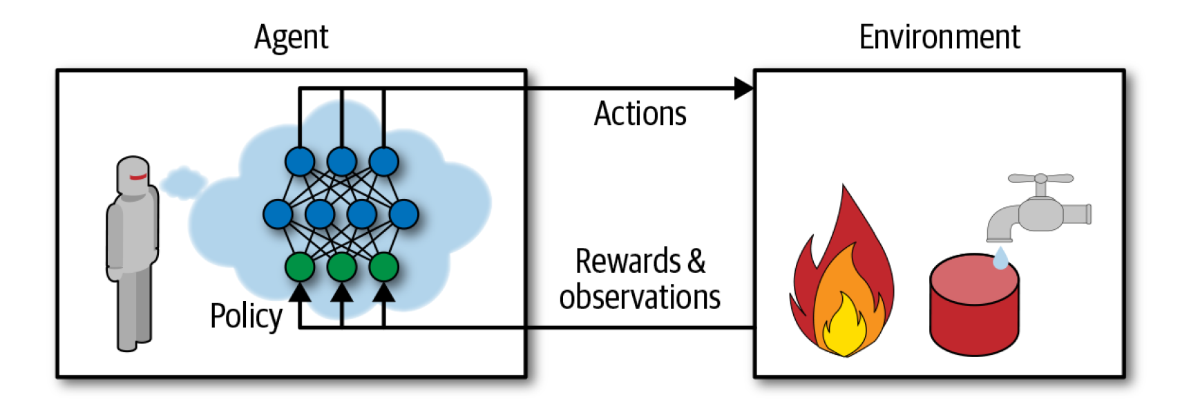
In short if I have to explain but will also give a brief overview of what actually Reinforcement Learning does is that there is a software agent. This “agent” can be the program controlling robots, playing a board game such as Go. What this agent does is it makes observations within an environment and takes actions according to the observations taken. In return, the agent receives rewards. If the “actions” taken are the right one, the agent will receive positive reward and if not, it will receive negative rewards. Now, you must be getting one question: how this agent determines its action whether it will give positive reward or a negative one. The answer is clear and many would have guessed it till now, it is the algorithm which is the set of instructions to achieve a particular task. In Reinforcement Learning, this algorithm is named as POLICY. It basically takes “observations” as input and gives “actions” as output.

Now, let’s consider, we have to balance the pole on a moving cart. How can we achieve this? As previously said, we will be needing an algorithm to train the system so that the pole could balance on a moving cart. There are different approaches to this but here I will present you with a Hard Coded Policy and a well known optimization technique called Policy Gradients.

OpenAI Gym

Before coming to Policy Gradients, one of the challenges of Reinforcement Learning is that in order to train an agent, you first need to have a working environment. If you want to program a walking robot, then the working environment is the real world and training in the real world has many repercussions, so we need a simulated environment and OpenAI Gym serves the purpose at its best. OpenAI Gym is a great toolkit for training agents, developing and comparing Reinforcement Learning algorithms. It provides many simulated environments(Atari games, board games, 2D and 3D physical simulations) for your learning agents to interact with.

To run a Gym in a colab, you have to install prerequisites like xvbf, opengl & other python-dev packages. For rendering the environment, you can use pyvirtualdisplay. This is clearly mentioned in my repo. Head over to this link and get it done, it is shown in Colab Preambles part of the code: OpenAI Gym prerequisites

Imports

To start working with CartPole Environment, we have to first import all the python packages required. Head over to this link and get it done, it is shown in Setup and Introduction to OpenAI gym part of the code: Setup

CartPole Environment

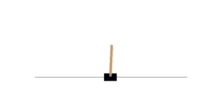
Create a CartPole environment. This is a 2D simulation in which a cart can be accelerated left or right in order to balance a pole placed on top of it. The agent must move the cart left or right to keep the pole upright. Create an environment with make().

After an environment is created, you must initialize it using the reset() method. This obs returns the first observation: Observations depend on the type of environment.

For the CartPole environment, each observation is a 1D NumPy array containing four floats: these floats represent the cart’s horizontal position (0.0 = center), its velocity (positive means right), the angle of the pole (0.0 = vertical), and its angular velocity (positive means clockwise).

Let’s plot the current observation:

Let's see how to interact with an environment. Your agent will need to select an action from an action space (the set of possible actions).

Discrete(2) means that the possible actions are integers 0 and 1, which represent accelerating the cart left (0) or right (1).

Now, we can make use of this action space to play with the cart-pole environment.

The cart is now moving toward the right (obs[1] > 0). The pole is still tilted toward the right (obs[2] > 0), but its angular velocity is now negative (obs[3] < 0), so it will likely be tilted toward the left after the next step.

The step() method executes the action and returns 4 values:

• obs - This gives the observation as previously explained.
• reward - This gives the reward at every step. You will get 1 point reward at each step.
• done - This will be “True” when one episode will be over. An episode is a bunch of steps or the sequence of steps between the moment the environment is reset until it is done is called an episode(For example - 10 steps == 1 episode).
• info - This will give some extra information that may help in debugging or in training.

Hard Coded Policy

Let’s move on to the main business, training the model so that the pole could balance itself on a moving cart. First, we will train our model with a policy which is hard-coded. This will be a simple policy that accelerates the cart left when the pole is leaning toward the left and accelerates the cart right when the pole is leaning toward the right. We will run this policy to see the average rewards it gets over 500 episodes:

This is the hard coded policy:

From the output, we can see that np.max(totals) return 68. Even with 500 tries, this policy never managed to keep the pole upright for more than 68 consecutive steps. Not great. If you look at the simulation, you will see that the cart oscillates left and right more and more strongly until the pole tilts too much.

Neural Network Policy

The hard coded policy didn’t work to the expectations as this environment is considered solved when the agent keeps the poll up for 200 steps.

So, we will be creating a Neural Network Policy which will take observation as input and it will output the action. It will estimate a probability for each action and then you will select an action randomly according to the estimated probability. In a CartPole environment where there are two actions(left or right), you will need just one output neuron which will output the probability p of action 0(left) and the probability of action 1(right) will be 1-p. The CartPole problem is simple as the observations are noise-free meaning that if the observation has some noise then in that case you have to use the past few observations to estimate the most likely current state. They also contain the environment’s full state meaning that it has no hidden state like if the environment only revealed the position of the cart but not it’s velocity, you would have to consider not only the current observation but also the previous observation in order to estimate the current velocity.

Here is a simple Sequential model to define the neural policy network:

Policy Gradients

While evaluating actions, there comes a popular problem known as the credit assignment problem. In Reinforcement Learning, the only guidance the agent gets is through rewards. But these rewards are sparse and delayed. Consider this example, if the agent manages to balance the pole for 50 steps, then we actually don’t know due to which particular action the pole gets unbalanced. We are only aware of that due to the last action it must have been unbalanced but this is not the truth because the previous actions have also been responsible for the cause.

To tackle this problem, we will be needing this Policy Gradient algorithm. Basically, it optimizes the parameters of a policy by following the gradients toward higher rewards. The process is:

• The neural network policy is allowed to play the game several times, and at each step, gradients are computed that would make the chosen action appear more likely.

  NOTE - Do not apply this gradient now, keep it for further use.

• After running several episodes, an action’s advantage is computed. The question is how it is calculated: For a particular action, the sum of all the rewards are calculated that comes after it by applying discount factor Y(Gamma) at each step. Consider this, if an agent decides to move right three times. By doing so, it receives +20 reward after the first step, 0 after the second step and -40 after the last one. Using discount factor of Y=0.8, the first action will have a return of 20 + Y*0 + Y^2 *(-40) = -5.6. The problem is that a good action can be followed by several bad actions which may lead to the good action getting a low return, but if we run the game enough times, good actions will receive higher returns on average. This is done by normalizing all the action returns by subtracting the mean and dividing by the standard deviation.
• The particular action was probably good if it’s advantage is positive. The gradients computed earlier is used here to make the action appear more likely. If it is negative then the opposite gradients are used to make that action appear less likely in the future. We just have to multiply each gradient vector by the corresponding action’s advantage.
• Lastly, the mean of all the resulting gradient vectors are computed and used to perform a Gradient Descent Step.

Let us use tf.keras to implement this algorithm: We will start with creating a play_one_step() function which will play the action for one step.

Let us see what this lines of code does:

• This code starts with a function to play one step at a time. Within the GradientTape block, the model is being called giving a single observation which will output the probability of going left.
• In the next line, we sample a random float between 0 and 1 and put a condition whether it is greater than left_proba. If left_proba is high, the action will be most likely False, if left_proba is low, the action will be most likely True.
• Next, we define the target probability(y_target) of going left which is 1 minus the action(cast to a float). If the action computed is 0(left), then the target probability of going left will be 1 which is True. If the action is 1(right), then the target probability will be 0 which is False.
• Next, we compute the loss using the loss function(loss_fn) and we use the tape(tape.gradient) to compute the gradient of the loss with model trained variables which will be tweaked later depending on how good or bad the action was.
• Finally, we play the selected action and we return the new observation, reward, done and info using step() method.

Now, we have to create another function play_multiple_episodes() which will depend on the play_one_step() function and will play multiple episodes. This code will return a list of reward lists (one reward list per episode, containing one reward per step), as well as a list of gradient lists (one gradient list per episode, each containing one tuple of gradients per step and each tuple containing one gradient tensor per trainable variable).

The Policy Gradient algorithm will use this play_multiple_episodes() function to play the game several times, then it will go back and look at all the rewards, discount them and normalize them as previously mentioned.

To discount and normalize, we will need two more functions:

The first one is the discount_rewards() function which will compute the sum of future discounted rewards at each step.

The second one is the discount_and_normalize_rewards() function which will normalize all the previously computed discounted rewards across many episodes by subtracting the mean and dividing by the standard deviation.

Let me show you what actually happens with these two functions:

• discount_rewards() - Let’s consider, there were 3 actions, and after each action there was a reward: first 10, then 0, then -50. If we use a discount factor of 80%, then the 3rd action will get -50 (full credit for the last reward), but the 2nd action will only get -40(0 + (0.8) * (-50)), and the 1st action will get -22(10 + (0.8) * 0 + (0.8)^2 * (-50)).



discount_rewards([10, 0, -50], discount_rate=0.8)


OUTPUT

array([-22, -40, -50])



• discount_and_normalize_rewards() - We compute all the mean and standard deviation of all the discounted rewards and we subtract the mean from each discounted reward, and divide by the standard deviation. Let’s consider, there are two episodes of 3 and 2 steps each. When we compute it, we can see that the normalized rewards(action’s advantage) is negative for the first episode and positive for the second episode. So, the actions from the second episode will be considered good.



discount_and_normalize_rewards([[10, 0, -50], [10, 20]], discount_rate=0.8)


OUTPUT

[array([-0.28435071, -0.86597718, -1.18910299]), array([1.26665318, 1.0727777 ])]

Now, we are almost ready to run the algorithm. Some things are still required. Those are the hyperparameters.

This will run 150 training iterations, will play 10 episodes per iteration, and each episode will last at most 200 steps. We will use a discount factor of 0.95.

We will need an optimizer and loss function. We will take Adam optimizer with learning rate 0.01 and binary cross-entropy loss function because we are training a binary classifier.(two possible actions: left or right)

Let’s move forward and run the training loop:

Let us see what this lines of code does:

• At each training iteration, the for loop calls the play_multiple_episodes() function which plays the game 10 times(n_episodes_per_update) and returns all the rewards and gradients for every episode and step.
• Next, we call the discount_and_normalize_rewards() function to compute each action’s normalized advantage(final_reward).
• Then, we have a for loop for model trainable variables which will compute the weighted mean of the gradients for that variable over all episodes and all steps, weighted by the final_reward.
• At last, we apply the mean gradients using the optimizer. This way, the model’s trainable variables will be tweaked and the policy is all ready to balance the pole on the moving cart.

Hurray, we trained our neural network policy and we are ready to see how well it is trained through the animation:

Just reading makes it boring I know that because I myself get bored, so just head over to the code in my repo and try it out. Here is the link: A Tour of Policy Gradients

You will surely enjoy this

Thank you.